Identifying NBA Shot Times Using Tracking Data
Data + Abstract
This article uses NBA tracking data provided by SportVU that can be found in this github repository. There are other articles on my website that discuss the use and limitations of this data, but I will give a brief refresher. It is 25 Hz tracking data that provides the \((x,y)\) locations of the 10 players on the court and the ball, the height of the ball above the court is also provided. It comes pre-packaged with play-by-play data and shot logs similar to the ones that can found using the NBA API here.
A follow up article discussing improvements to the methodology can be found here.
The play-by-play data comes from live-scoring performed by statisticians during the game, and (as someone who has worked in live-scoring) I can attest that recording the precise time of events is not what you are focused on in the middle of a game. Often times it takes a couple extra seconds to see the outcome of a shot before the event is officially recorded. As such, this repository comes with setup to fix those reported shot times to the precise moment the ball leaves the shooters hand. The Problem: The built in setup function doesn't work. Somewhat of an exaggeration; inconsistent may be a better word. When the legacy function works it works exactly as intended, but it doesn't always work. Duplicate shot times, duplicate shot locations,... I've covered this in previous articles, so I will now continue to explaining how the "fix_shot_times" builtin is designed to function.
If you don't like geeking out over math then feel free to skip this section after the next two sentences. In summary: the built-in function finds the shot time by identifying when the ball's vertical acceleration is greatest. Makes sense, right? When a player takes a shot the ball quickly ascends, so if we find when that ascent begins that would be the time the shot was taken. Now lets breakdown how this methodology is implemented in practice.
The Savitzky-Golay Filter
The primary purpose of the Savitzky-Golay filter is to smooth noisy data without distorting the true signal. Here's how it works.
Suppose we have a set of data points
\[ \{(x_i,y_i)\}, \quad i=1,\dots,N \]We aim to fit a polynomial of degree \(p\) to these points. The polynomial can be expressed as
\[ y = a_0 + a_1 x + a_2 x^2 + \dots + a_p x^p \]For a given window centered on \(x_k\), we determine coefficients \(a_0, a_1, \dots, a_p\) such that the polynomial fits the data points in the window.
This is achieved by minimizing the sum of squared differences between the observed values and the polynomial prediction.
\[ \min \sum_{i=-m}^{m} \left( y_{k+i} - \sum_{j=0}^{p} a_j x_{k+i}^{\,j} \right)^2 \]The window size is 2m + 1 centered at \( x_k\)
---Example
Consider a window size of 5 (\(m=2\)) and a polynomial degree of 2 (\(p=2\)).
The data points in the window are
\[ (x_{k-2},y_{k-2}), (x_{k-1},y_{k-1}), (x_k,y_k), (x_{k+1},y_{k+1}), (x_{k+2},y_{k+2}) \]We fit the polynomial
\[ y = a_0 + a_1 x + a_2 x^2 \]by minimizing
\[ \min \sum_{i=-2}^{2} \left( y_{k+i} - (a_0 + a_1 x_{k+i} + a_2 x_{k+i}^2) \right)^2 \]
After determining the coefficients (for example using
scipy.optimize), the smoothed value at \(x_k\) is
Code Implementation
def sg_filter(x, m, K=0):
    # X = time window
    # m = polynomial degree
    # K = derivative order
    mid = len(x)//2
    # center the window around the midpoint
    a = x - x[mid]
    # construct powers of the centered variable
    expa = [a**i for i in range(0, m+1)]
    # design matrix (Vandermonde)
    A = np.array(expa).T
    # compute Moore-Penrose pseudo-inverse
    Ai = np.linalg.pinv(A)
    # each row corresponds to a filter kernel
    return Ai[K]
The pseudo-inverse used above is
\[ A^+ = (A^T A)^{-1} A^T \]Each row of \(A^+\) corresponds to a set of filter weights.
- \(K=0\): smoothing (estimate position)
- \(K=1\): first derivative (velocity)
- \(K=2\): second derivative (acceleration)
When the weights are dotted with the local window of \(y\)-values, value = np.dot(weights, y_window) ,the result is the smoothed or derivative
estimate at the center point.
Since tracking data tends to be noisy, and all data points are equally spaced (40 milliseconds apart), a Savitzky-Golay filter is ideal for our uses. We utilize the additional benefit that the resulting polynomial is differentiable to find instantaneous vertical acceleration of the ball in order to determine shot times.
Application to Tracking Data
Applying an SG filter to tracking data, we fit a curve to the balls height as a function of game clock. Then the greatest moment of vertical acceleration is taken as the shot time, and the \((x,y)\) coordinates of the ball at that time are taken as the shot location. Here is the original implemtation to fix shot times with an example case.
def correct_shots(game_shots, movement, events):
  fixed_shots = pd.DataFrame(columns=game_shots.columns)
  for ind, shot in game_shots.iterrows():
    try:
        event_id = shot["GAME_EVENT_ID"]
        movement_around_shot = movement.loc[
            movement["event_id"].isin([event_id, event_id - 1])
        ].drop_duplicates(subset=["game_clock"])
        game_clock_time = movement_around_shot.query("team_id == -1")[
            "game_clock"
        ].values
        ball_height = movement_around_shot.query("team_id == -1")["radius"].values
        size = 10
        order = 3
        params = (game_clock_time, ball_height, size, order)
        position_smoothed = smooth(*params, deriv=0)
        acceleration_smoothed = smooth(*params, deriv=2)
        max_ind = np.argmax(position_smoothed)
        shot_window = acceleration_smoothed[max(0, max_ind - 25) : max_ind]
        shot_min_ind = np.argmin(shot_window)
        shot_ind = max_ind - shot_min_ind
        shot_time = game_clock_time[shot_ind]
        quarter = movement_around_shot["quarter"].values[0]
        movement_around_shot = movement_around_shot.query(
            "game_clock == @shot_time"
        )
        shot["QUARTER"] = quarter
        shot["SHOT_TIME"] = shot_time
        shot["LOC_X"] = movement_around_shot.query("team_id == -1")["x_loc"].values[
            0
        ]
        shot["LOC_Y"] = movement_around_shot.query("team_id == -1")["y_loc"].values[
            0
        ]
    except Exception:
        continue
    # fixed_shots = fixed_shots.append(shot)
    fixed_shots = pd.concat([fixed_shots, pd.DataFrame([shot])], ignore_index=True)
  return fixed_shots
Example:
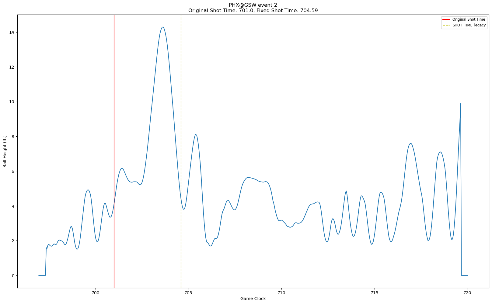
We can observe that the legacy version of the function is able to correctly identify the moment when the ball
begins accelerating upwards towards the hoop. A visual confirmation from the game film confirms this.
The Problem:
To see the problem with the legacy version of the function, lets look at the same graph for the very next
possession:
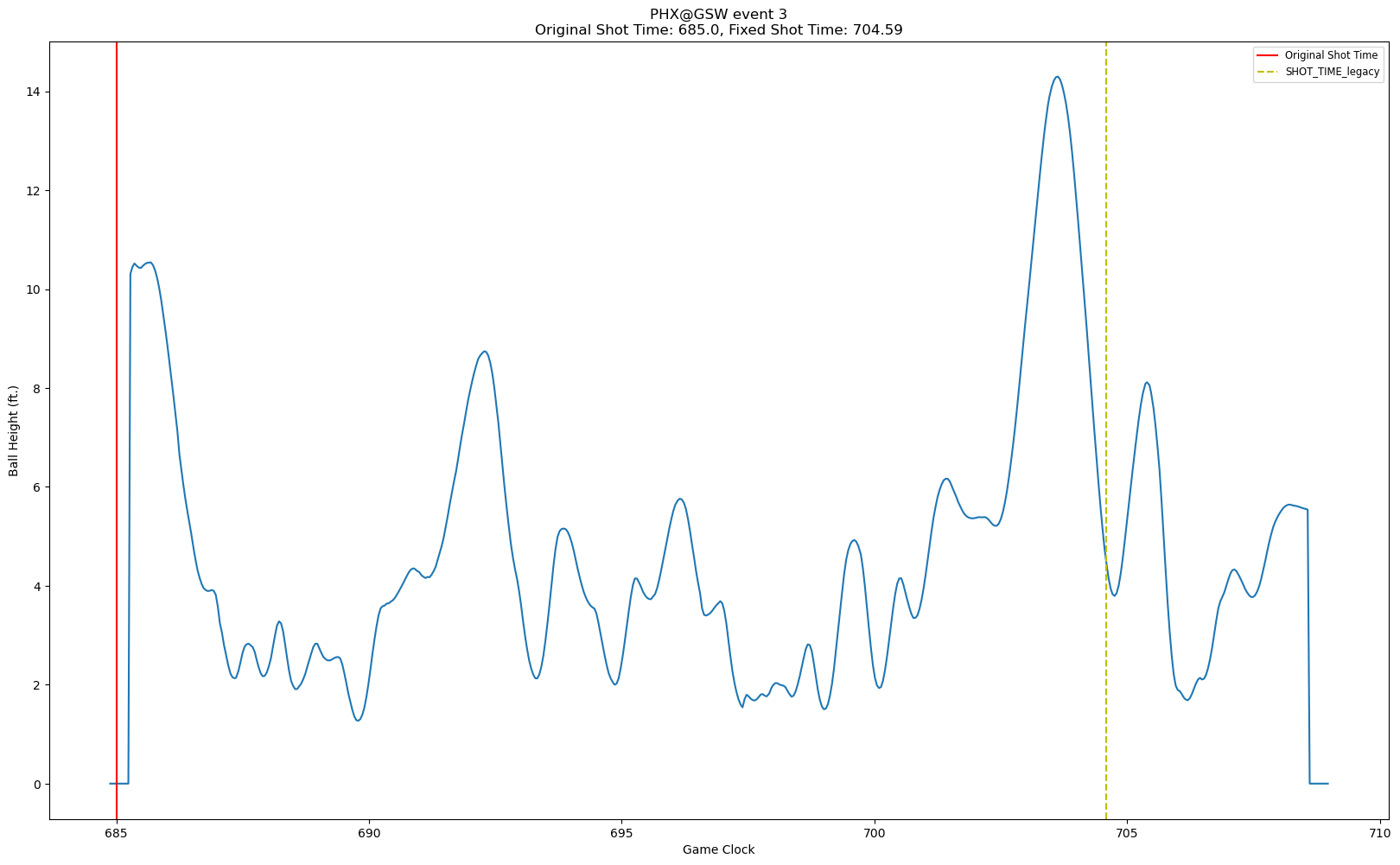 The function returned the same value for shot time despite the second shot being taken nearly 15 seconds later
because the window of movement data extends from the previous possession! Because the signal from the first shot
is stronger, the function only sees that instead of the signal from the second shot. The astute among you may
have noticed that the original function considers data from the previous possession, so you would immediatly
suggest to simply filter for the specific event ID assosciated with the shot. That is good intuition, but it
will unfortunately we see that will not fully address the issue if we examine the tracking data. Below is a
sample of the tracking data from PHX@GSW, filtered for game clock = 704.59 in the first quarter:
The function returned the same value for shot time despite the second shot being taken nearly 15 seconds later
because the window of movement data extends from the previous possession! Because the signal from the first shot
is stronger, the function only sees that instead of the signal from the second shot. The astute among you may
have noticed that the original function considers data from the previous possession, so you would immediatly
suggest to simply filter for the specific event ID assosciated with the shot. That is good intuition, but it
will unfortunately we see that will not fully address the issue if we examine the tracking data. Below is a
sample of the tracking data from PHX@GSW, filtered for game clock = 704.59 in the first quarter:
| index | event_id | game_clock | team_id | player_name | x_loc | y_loc |
|---|---|---|---|---|---|---|
| 6666 | 2 | 704.59 | -1 | ball | -23.3061 | 157.13 |
| 9966 | 3 | 704.59 | -1 | ball | -23.3061 | 157.13 |
As we can see, the reason that the fix_shot_times won't work as intended is because the tracking data has duplicate rows which have the same values for game clock, but different values for event ID. Generally, this is actually good because it could be useful to have information on the locations of players for large stretches of time around each event, so that if examining a specific event you get information on the surrounding movement
Our first thought may be to drop these duplicate rows that have the same value in the game_clock column and call it a day. But like I said above, it could be beneficial to have info about movement before/after events. Also there are stretches of the game where the shot clock stays the same but players are still moving (inbounding plays etc…), and we definitely don't want to lose that information by unilaterally dropping duplicate rows. In a future article I will explore how to improve this methodology.
-Nick