Calculating Offensive Versatility Score in Python
In this post I am going to walk through the process of computing Offensive Versatility Score. From collecting the data all the way to the finished product. All data is courtesy of basketball-reference. Linked directly below is the original OVS post on this site where all the data and rankings can be found.
The first step is to collect and merge all the data that we will need. Here I am scraping additional data so that I can do more advanced analysis, but only the shooting data is required for computing OVS. I am going to be doing this in Python because it is the language I am most skilled with. This is actually the first time I've ever done this, and it is a HUGE improvement. Usually I do this in excel using custom built macros, but getting the data into Python ended up not being that difficult and I will likely continue using this method going forward.
To do this I used Pandas, Numpy, Time, and Matplotlib + Seaborn for visualizations. Pandas has a built in webs craping tool which I found to be more effective than using BeautifulSoup, Selenium, or other web scraping modules. We need to include the Time module to not exceed the web scraping limits that basketball-reference has in place internally. If you're not totally versed in coding, that's ok! You can follow along with the logic using the comments (the lines that start with ##).
      ##For each year for which shooting/play-by-play data is available (1997-)
      for year in range(1997,2025):
          ##Get total counting stats page
          totals_url = f'https://www.basketball-reference.com/leagues/NBA_{year}_totals.html'
          ##pd.read_html() returns a list, our list will only have one element so we take that one
          totals_df = pd.read_html(totals_url, header=0, attrs={'id':'totals_stats'})[0]

          ##Get shooting stats page
          shooting_url = f'https://www.basketball-reference.com/leagues/NBA_{year}_shooting.html'
          ##Shooting has a double header so we start at index 1
          shooting_df = pd.read_html(shooting_url, header=1, attrs={'id':'shooting'})[0]
          ##Drop columns we don't need
          ##'Rk', 'Pos', 'G', 'GS', 'MP' ,'Age' ,'FG%' ,'Awards' are duplicates
          ##'Dist.', '2P', '2P.1', '%FGA', '#', 'Att.', 'Md.' are not that useful to us
          shooting_df = shooting_df.drop(columns=[
              'Rk', 'Pos', 'G', 'GS', 'MP', 'Age', 'FG%', 'Dist.', '2P', '2P.1', '%FGA', '#', 'Att.', 'Md.', 'Awards'
          ])
          ##Rename columns for clarity, Pandas appends '.1' to duplicate column names
          ##The first five distance ranges are frequency and the dupes are FG% for each range respectively
          shooting_df = shooting_df.rename(columns={
              '0-3':'0-3f', '3-10':'3-10f', '10-16':'10-16f', '16-3P':'16-3Pf', '3P':'3Pf',
              '0-3.1':'0-3FG%', '3-10.1':'3-10FG%', '10-16.1':'10-16FG%' ,'16-3P.1':'16-3PFG%' ,'3P.1':'3PFG%',
              '2P.2':'2P-astd', '3P.2':'3P-astd', '%3PA':'Corner3-Rate', '3P%':'Corner3-FG%'
          })

          ##Get advanced stats page
          advanced_url = f'https://www.basketball-reference.com/leagues/NBA_{year}_advanced.html'
          advanced_df = pd.read_html(advanced_url, header=0, attrs={'id':'advanced'})[0]
          ##Drop columns we don't need
          ##'Rk', 'Pos', 'G', 'GS', 'MP', 'Age', 'Awards', '3PAr' are all duplicates
          advanced_df = advanced_df.drop(columns=['Rk', 'Pos', 'G', 'GS', 'MP', 'Age', 'Awards', '3PAr'])

          ##Get play-by-play stats page
          pbp_url = f'https://www.basketball-reference.com/leagues/NBA_{year}_play-by-play.html'
          ##Play-by-play has a double header so we start at index 1
          pbp_df = pd.read_html(pbp_url, header=1, attrs={'id':'pbp_stats'})[0]
          ##Drop duplicate columns
          pbp_df = pbp_df.drop(columns=['Rk', 'Pos', 'G', 'GS', 'MP', 'Age', 'Awards'])
          ##Rename columns for clarity
          pbp_df = pbp_df.rename(columns={'Shoot':'Shoot_commited', 'Off.':'Off_commited', 'Shoot.1':'Shoot_drawn',
                                        'Off..1':'Off_drawn', 'PGA':'PointsGeneratedAssists'})

          ##Pandas only allows merging two dataframes at a time, so we merge in pairs then merge the pairs
          df1 = pd.merge(totals_df, shooting_df, on=['Player','Team'], how='outer')
          df2 = pd.merge(advanced_df, pbp_df, on=['Player','Team'], how='outer')
          data_df = pd.merge(df1, df2, on=['Player','Team'], how='outer')

          ##Write the data to a csv file so I never have to do this again
          data_df.to_csv(f'Data-April-10-2025/{year}-stats.csv', index=False)

          ##Print an update statement
          print(f'Data from {year} successfully scraped')

          ##Sleep the system for 20 seconds to not exceed basketball-reference scraping limits of 20 scrapes / 60 seconds
          ##20 second sleep => 12 scapes / 60 seconds which will keep me under the limit
          time.sleep(20)
Now I'm going to load the data back in so we have access to everything without needing to worry about corrupting the data or repeatedly scraping the site. I define a dictionary, which allows us to access the data for whichever year(s) we want.
      ##Define a dictionary to store the data for each year
      data = {}
      for year in range(1997,2025):
          data[f'{year}'] = pd.read_csv(f'Data-April-10-2025/{year}-stats.csv')
          print(f'Data from {year} successfully read')
Now for the good stuff: calculating some stats! The first thing we are going to do is calculate non-position adjusted OVS
        ##Setting a minimum attempts filter which we can fine-tune later
        min_attempts = 100
        ##First off lets calculate crude OVS and assist/turnover ratio for each year
        for year, df in data.items():
            ##Assist to turnover is pretty quick and easy to calc
            df['AST/TOV'] = df['AST'] / df['TOV']

            ##We want to calculate league averages from among players who have taken a minimum amount of shots
            qualifiers = df.loc[df['FGA'] >= min_attempts]
            ##Calculate league average frequency and FG% among qualifiers
            league = qualifiers[
                ['0-3f', '3-10f', '10-16f', '16-3Pf', '3Pf', '0-3FG%', '3-10FG%', '10-16FG%', '16-3PFG%', '3PFG%']
            ].mean()
            ##When we make the calculation it will be for all players, including non-qualifiers, which we can filter later


            ##Define shot ranges as a list for quicker looping
            shot_ranges = ['0-3', '3-10', '10-16', '16-3P', '3P']
            ##Find partial OVS scores for each range
            for shot_range in shot_ranges:
                df[f'{shot_range} Score'] = (
                    df[f'{shot_range}f'] / league[f'{shot_range}f']
                ) * (
                    df[f'{shot_range}FG%'] / league[f'{shot_range}FG%']
                )

            ##Take the average of the scores for each range and boom, crude OVS!
            df['OVS'] = df[[f'{sr} Score' for sr in shot_ranges]].mean(axis=1)
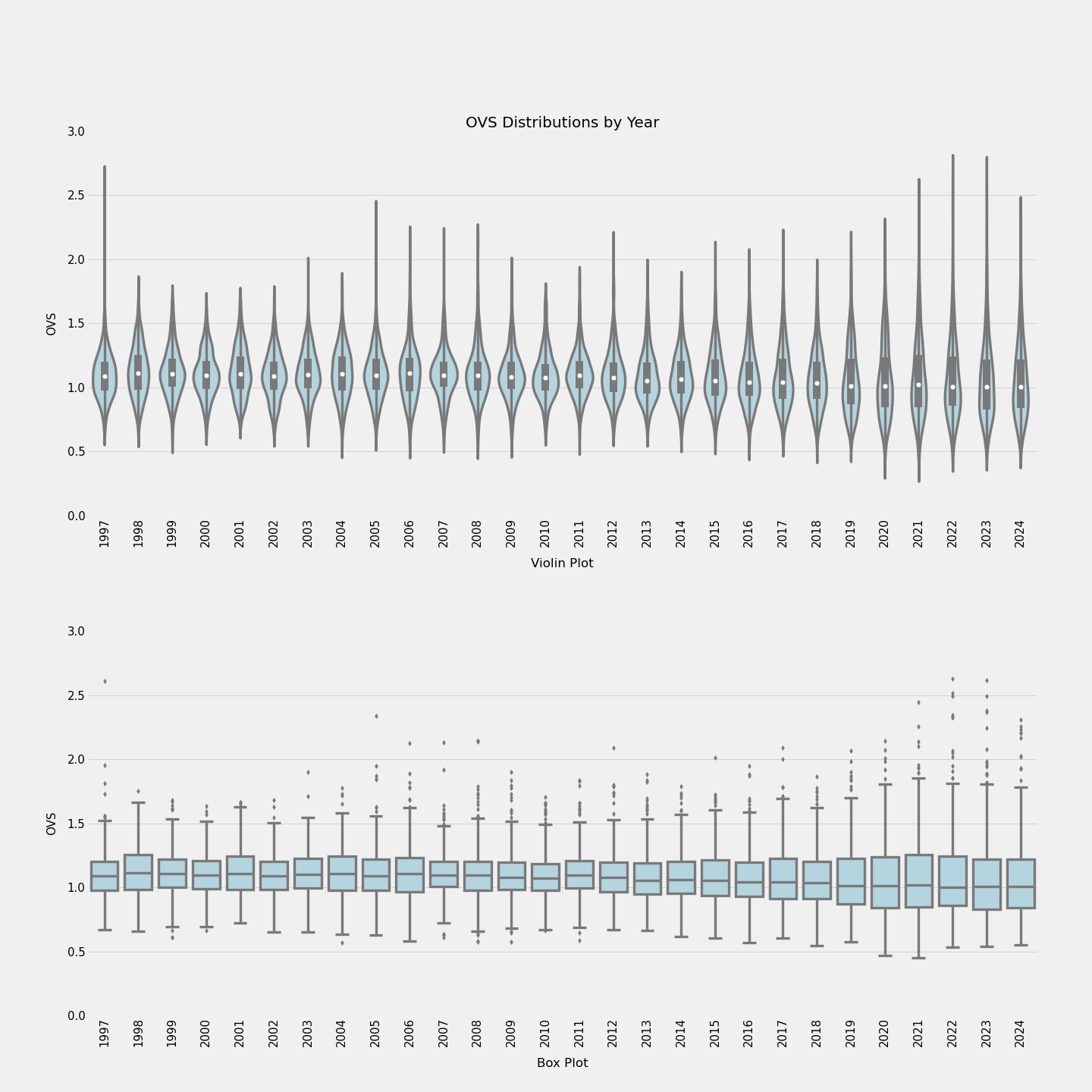
It's tempting to immediatly, but first lets get a sense of the data with a few visualizations. I like to use violin plots because they show summary statistics like the median and quartiles as well as the density of the data. I also included traditional box and whiskers plots because violin plots have a weakness when it comes to showing outliers. And this decision is also justified in the comments of the code used to generate this figure. Only players at or above the minimum shot attempts are included in the figure.
        ##Lets visualize summary statistics for all years side by side
        ##I like to use violin plots because they give us summary information (median, quartiles), and also let us get a
        ## sense of distribution.
        ##We need to combine all OVS values from the dictionary into one dataframe
        records = []
        for key, df in data.items():
            ##Looking at only the players who are above the minimum value of attempts
            qualifiers = df.loc[df['FGA'] >= min_attempts]
            for val in qualifiers['OVS']:
                records.append({'Group': key, 'OVS': val})
        OVS_df = pd.DataFrame(records)
        ##Set up some plots
        fig, axes = plt.subplots(2, 1, figsize=(24, 24), dpi = 60)
        ##Plot all violins side by side
        sns.violinplot(
            data=OVS_df,
            x='Group',
            y='OVS',
            inner='box',
            color='lightblue',
            ax = axes[0]
        )
        ##Lets make it look better
        axes[0].set_title('OVS Distributions by Year', fontsize=24)
        axes[0].set_ylabel('OVS', fontsize=18, labelpad=15)
        axes[0].set_xlabel('Violin Plot', fontsize=20, labelpad=18)
        axes[0].set_ylim(0, 3)
        axes[0].tick_params(axis='x', rotation=90, labelsize=18)
        axes[0].tick_params(axis='y', labelsize=18)
        ##These are good, but the long necks on each violin tell me there are probably a lot of outliers
        ## so lets use boxplots to get a better sense of those outliers
        ##Plot all boxplots side by side
        sns.boxplot(
            data=OVS_df,
            x='Group',
            y='OVS',
            color='lightblue',
            ax = axes[1]
        )
        ##Lets make it look better
        # axes[1].set_title('OVS Distributions by Year', fontsize=20) - We dont need to pass this again, one at the top is fine
        axes[1].set_ylabel('OVS', fontsize=18, labelpad=15)
        axes[1].set_xlabel('Box Plot', fontsize=20, labelpad=18)
        axes[1].set_ylim(0, 3)
        axes[1].tick_params(axis='x', rotation=90, labelsize=18)
        axes[1].tick_params(axis='y', labelsize=18)
        ##Final adjustments for beautification
        fig.subplots_adjust(hspace=0.3)
        plt.savefig('crude_OVS.png')
        plt.show()
This is good, unequivocally. Outliers are almost limited, and indeed expected. In my opinion having outliers in sports data in good and normal. They greatest players are by definition outliers in terms of athelticism, skill, etc.... A good observation to make here is that as the years go on the density (represented by the width of each "violin") progressively gets skinnier. More on that later.
Now lets calculate a position adjusted version of OVS, OVS+. The process is largely the same, but league averages and scores are calculated respective to position (as according to basketball-reference). Here's the code:
        for year, df in data.items():
          qualifiers = df.loc[df['FGA'] >= min_attempts]
          ##Calculate league average frequency and FG% among qualifiers for each position
          league_pos = qualifiers.groupby('Pos')[
              ['0-3f','3-10f','10-16f','16-3Pf','3Pf','0-3FG%','3-10FG%','10-16FG%','16-3PFG%','3PFG%']
          ].mean()
          ##When we make the calculation it will be for all players, including non-qualifiers, which we can filter later
          ##Define positions for looping
          positions = ['PG','SG','SF','PF','C']
          ##Define shot ranges for looping
          shot_ranges = ['0-3','3-10','10-16','16-3P','3P']
          ##For each position we calculate OVS
          for position in positions:
              pos_df = df.loc[df['Pos'] == position].copy()
              ##Find partial OVS+ scores for each range
              for shot_range in shot_ranges:
                  pos_df[f'{shot_range} Score+'] = (
                      pos_df[f'{shot_range}f'] / league_pos.loc[position][f'{shot_range}f']
                  ) * (
                      pos_df[f'{shot_range}FG%'] / league_pos.loc[position][f'{shot_range}FG%']
                  )
                  df.loc[df['Pos'] == position, f'{shot_range} Score+'] = pos_df[f'{shot_range} Score+']
              ##Take the average of the scores for each range, throw it back to the original dataframe and kapow!
              df.loc[df['Pos'] == position ,'OVS+'] = pos_df[[f'{sr} Score+' for sr in shot_ranges]].mean(axis=1)
Let's take a look at the same visualization for the newly calculated rendition:
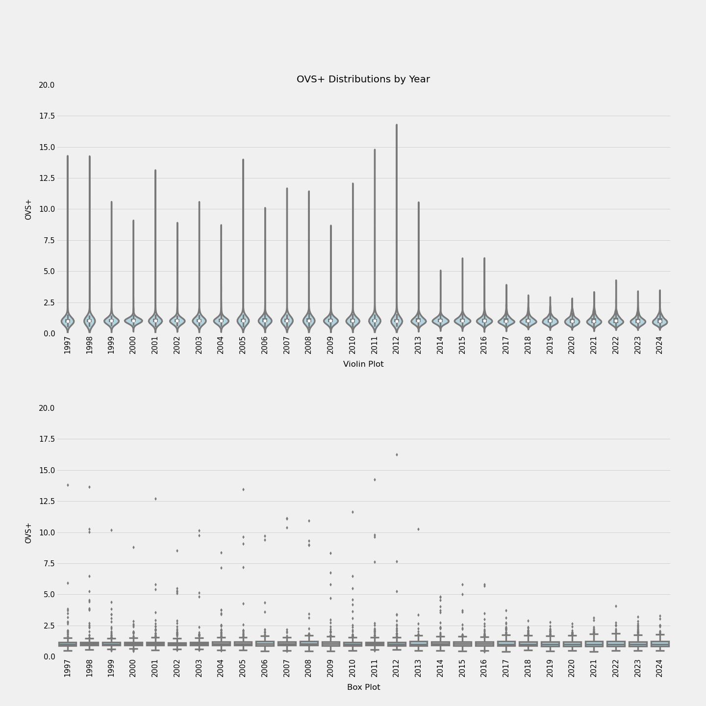
Woah. Right off the bat this data is obviously (Charles Barkley voice) terribly skewed. So lets break down it down. Our violin and box immediatly show that we have extreme outliers, to a much higher degree than in crude OVS. I took a closer look at 2012 since it had the most extreme outlier among all years, and found exactly what I expected: a OVS+ ranking dominated by bigs. Of the top 25, 23 were either centers or power forwards. Notable exceptions are Shaun Livingston, the poster boy of midrange masters, and Evan Turner who also knew how to get his in the midrange. Kurt Thomas is another interesting one. The statistical signal that we get from him is that of a relic of a lost age. He didn't shoot any threes, but he was still shooting those long 2's that were losing favor around the league. Looking at the correlations between variables, we see that OVS+ is almost completely determined by 3P Score+.
Another interesting trend, which can be observed looking at the violin plot, is the distribution throughout the years. It is not a coincidence that the last eight years have the smallest distribution of values. Can we think of anything or anyone that may have fundamentally changed the way the game is played circa 2016? Perhaps in the western conference? Perhaps wears #30? Last name Curry? No? Me niether. Since then the NBA has also had a positionless revolution, which heavily contributed to the meager normalization of OVS+ distributions recently. Even though these values have lost much of the practicality, the trend does suggest that the mathematical foundations of OVS are working correctly. In the years where bigs rarely stepped out and took shots from further away from the basket, those players could have provided incredible floor spacing, although that sort of spacing didn't become ubiquitously valued until more recent years.